Category Archives: Technology

General Tech

F Natural is Back

After a long hiatus I started teaching myself Python, and as a warm-up I wrote a little lambda interpreter in it. I was blown away by how convenient and quick it was in Python, and the project has kind of snowballed to the point where I have most of my previously only vapourware “F♮” functional language up and running (albeit only under a test harness.)

The source is GPL and on GitHub:  https://github.com/billhails/PyScheme

Singletons are NOT an anti-pattern

I get annoyed sometimes when beautiful patterns like the Null Object Pattern get dismissed out of hand because they use singletons. There is nothing wrong with singletons in themselves, the problem, and the anti-pattern, is when people use singletons to store global state. A good singleton, like the Null Object, keeps no (mutable) state and as such behaves as a constant, not a variable.

MVC – Man Vs. Computer

I confess, I’ve never done MVC before! I’ve heard about it and read about it of course, but just never had occasion to use it until now.

I run our arechery club’s website as a sort of a passtime. It’s enjoyable and relaxing and I’m not under any pressure to deliver anything. So I thought I would do a sightmarks calculator.

In case you’re not familiar with the finer points of archery, most bows have a sight attached. The sight is a vertical track marked in arbitrary units that sticks out in front of the bow and has a scope or a pin that can slide up and down the track for different distances. Archers have a little book of sightmarks that they keep, and write  down their sightmark for each distance. Now the amazing thing is that all that physics of ballistics and mathematics of trajectories seems to cancel itself out, so that there is a simple linear (or very nearly linear) relation between sightmark and distance.

All I wanted to achieve then, was a simple tool where an archer could enter a set of sightmarks and get a line of best fit for the data, which could then be used to generate a set of estimated sight marks for all the standard distances.

The tool would have an input section for the sample sightmarks,  a graph (canvas) showing the inputs and line of best fit, and a table of the resulting estimates.

It’s only slightly more complicated than that in practice because I wanted to be able to persist the data in the browser’s local storage, and to allow archers to save multiple sets of sightmarks for different bows, arrows and bow setups.

This is obviously screaming out for MVC. I didn’t want to add a dependency on any heavyweight javascript MVC framewaork, so I decided to write it from scratch. You can see the finished result at www.roystonarchery.org/new/sightmarks/ (apologies for the very slow site, it’s EIG.)

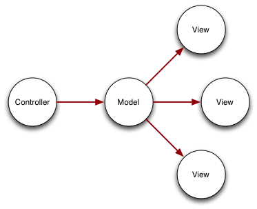
The basic idea of MVC is a Model which stores state, one or more Views which present the model to the user, and a Controller which allows manipulation of the model. Conceptually it’s as simple as:

MVC

I should point out that this is the original MVC pattern as espoused by SmallTalk80, not the more “modern” variants fitted to the web, but since this is a browser-only application that seems a reasonable choice of pattern.

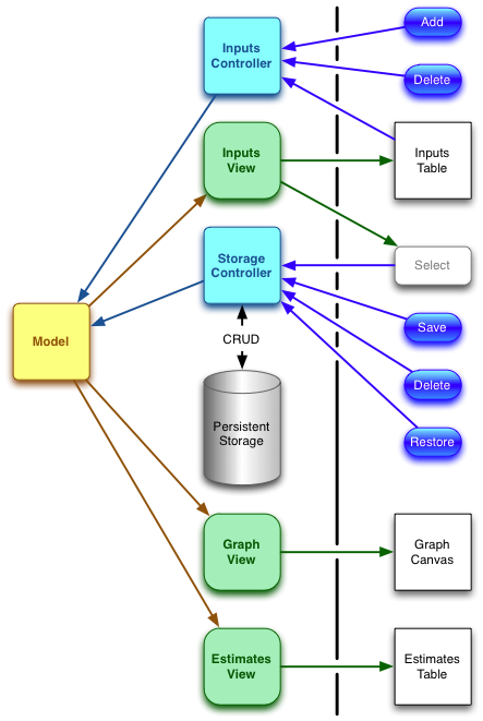
Of course real world programming is not that simple, and it took me an unreasonable amount of time to get this working. First of all I needed two controllers. The first would deal with the editing of the current model: adding and removing sight marks. The second controller would be concerned with persisting the data to local storage, restoring the data from local storage, and generally managing that data. The final architecture I came up with looks like this:

Sightmarks-MVC

The heavy vertical line demarcates user-visible components from the “back-end”.

It works quite well now, but I had a struggle to get there. Maybe it’s because I don’t know Javascript that well, and I’m only just learning jQuery and the DataTables API, but I think it’s more fundamental, that the MVC “pattern” is fundamentally flawed in that it is usually impossible not to blur the distinction between Model and Controller, or in my case between View and Controller.

The Storage Controller is fairly straightforward. It reacts to user input by saving and restoring the entire Model, and allows management of the storage directly (deleting unwanted sets of sightmarks.)

The Input controller was more difficult because it needs to take information from the displayed inputs (currently selected sightmark) in order to delete it from the model. I had to make some rules to stop the whole thing dissolving into mush.

Lessons Learned

The most important thing is to ensure that the only state kept is in the model. If there is any unavoidable secondary state (such as is maintained by the DataTables objects,) then that secondary state must be completely flushed and recreated by any change to the model, and should not be relied upon.

The second important thing is to resist the temptation to short-circuit the system by having controllers update views directly. To keep this thing sane, all communication between controller and view must go via the model.

Lastly, having a MVC structure is better than having no structure, but be prepared to have to twist things around to make it work.

MVC is a very old pattern, dating to the earliest SmallTalk systems in an age where user experience could take second place to a clean implementation. Nowadays the UX is paramount, and we may have to think again.

So You Feel Lucky?

I’ve just finished reading Stephen Jay Gould’s excellent book Wonderful Life (again) and it got me thinking about random trees.

In case you haven’t read it, Wonderful Life is about the fossil bed known as the Burgess Shales which contains extrordinarily well preserved fossils of soft and hard-bodied animals from a period just after the so-called Cambrian Explosion. The Cambrian Explosion marked the period when the seas first “exploded” with an enormous range of large, multicellular animals with hard shells that preserve easily. In the 1980s a detailed re-evaluation of the fossils found in the Burgess Shales provoked a scientific revolution in paleontology, because it turns out that only a small percentage of those fossils have any direct living descendants, and many of them represent previously unknown phyla (basic types of animals.) This did not fit comfortably with the established notion of evolution as ordered progress, with the basic groups of animals established early on and forming a predictable lineage all the way from microbe to man at the pinnacle. Rather it paints the picture of extinction being the norm, and the survival of one group or another very much in the hands of chance and historical contingency. The book is not an argument against Darwinism but rather a re-evaluation of some of its finer points. Crudely put, it’s not arguing against the existance of a Tree of Life, just questioning what shape the tree is.

Anyway with that in mind, and the somewhat vague hand-drawn trees in the book leaving my curiosity piqued, I started wondering what any real evolutionary tree might look like. Of course it’s impossible to ever produce an algorithm that will accurately represent a real evolutionary sequence, so I thought to keep it very simple.

We start with a “first progenitor“. It has two choices: form two new species or die out.

Each new species has the same option at the next toss of the coin. That’s it. In perl it would look something like this:


So there’s a 1/2 probability that the thing will never get started, and you’re left with a stump rather than a tree. But with 2 children, there’s only a ¼ chance that they will both die out, and if they both survive then there are 4 grandchildren, and so on. This code has a definite probability of running forever.

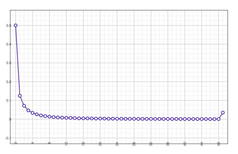
It turns out that if you run this a large number of times, and add up the  number of each depth reached, you get a curve that asymptotically approaches zero at infinity:

treegraph

The graph is normalized so the trees of depth zero come out at 0.5. The little kick at the right is those that reached the maximum depth in my test.

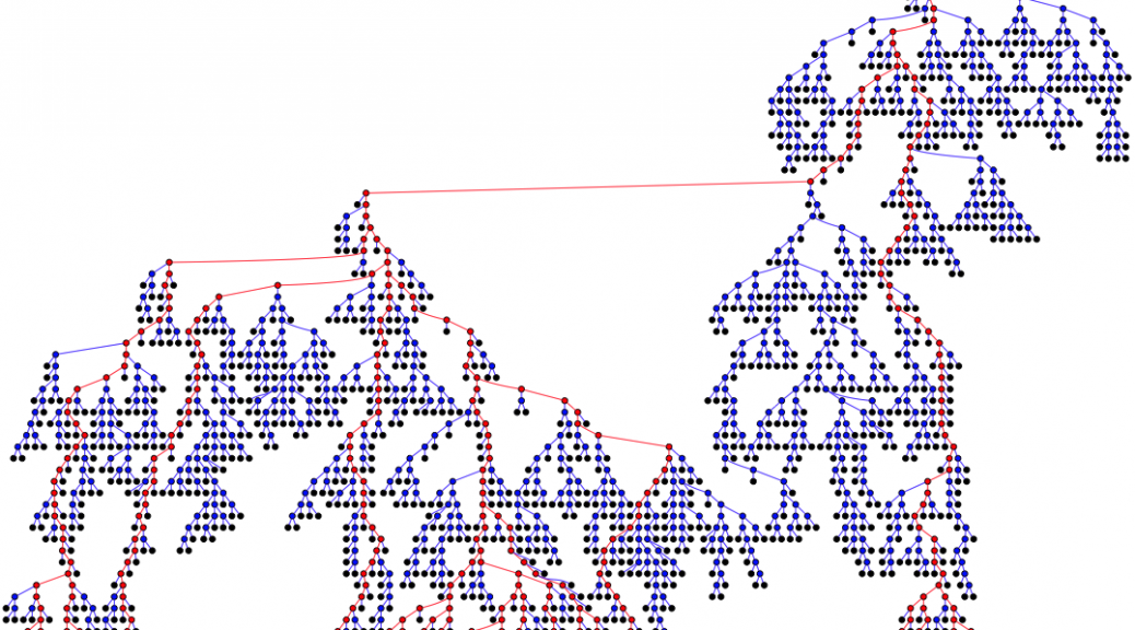
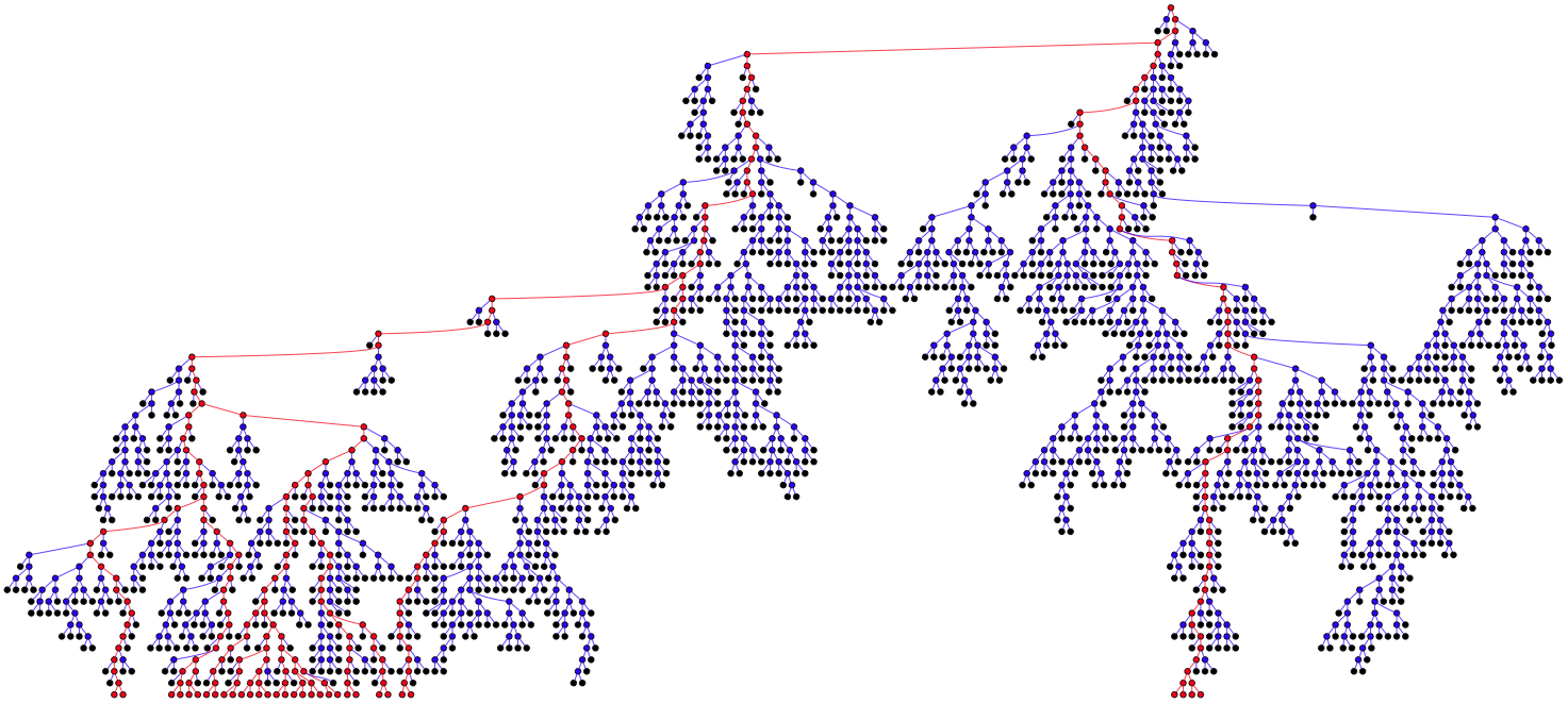
So what do these trees look like? I’ve given the game away by using a picture of one of them as the featured image for this post. As for generating the images, the excellent GraphViz comes to our rescue. With a little jiggery-pokery we can get the above perl code  to produce a .dot  file that we can feed to GraphViz and get a picture. I’ve extended the code to color nodes and vertices red if they are “survivors” (have descendents at the limiting depth) and black if they represent a species with no descendants. I’ve also changed the code to try again repeatedly until it generates a tree that reaches a limiting depth. Here’s a representative:

tree2

The limit was set at 60, so assuming 2 million years to create a species (I remember that figure from somewhere, I have a bad habit of throwing up unverified facts) this represents about 120,000,000 years of evolution from a single common ancestor. The interesting thing here I think is that the majority of branches don’t make it. Extinction is the norm, even for apparently large and flourishing branches. Apparently insignificant branches can suddenly flourish, and equally suddenly die out. I think this is close to Gould’s vision in general, if not in detail.

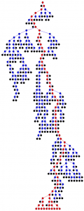
The other interesting thing is the huge variety of shapes. Some trees are wide, others are narrow, for example:

tree5

In this case all of the survivors share a common ancestor only a few generations (speciations) ago. This could easily be a model for the very earliest life, since the common ancestor of all current life on earth, who’s closest living relative is likely one of the Archaea, is far too complex to be a “first progenitor”.

I don’t know where I’m going with this from here, probably nowhere, but I think it’s interesting.

To finish off, here’s the full implementation of the tree generating code in case you want to try it yourself.  You can pick up GraphViz from www.graphviz.org and run it from the command-line (the commands are called dot , neato , circo  etc.) or via a gui.


The Y-Combinator

I’ve struggled a bit in the past to explain why letrec was necessary to allow recursion in a language with first class functions. All we’re trying to achieve is:

But without the use of a global subroutine name, or in fact any environment assignments. If you remember, letrec created a recursive function by creating a symbol naming the function first, with a dummy value,  then evaluated the function in the environment where it’s name was already present, then assigned the resulting closure to the symbol so the function could “see itself”. But in a purely functional setting, assignment is bad, right?

There is a little bit of programming language magic called the “Y-Combinator” that does the job. It’s very succinctly expressed in the λ calculus as:

That is to say, a function taking a function as argument  applying that function to itself, and given (a copy of) itself as argument.

In case this seems all a bit too esoteric, here it is in F♮:

And if that’s still too esoteric here it is in Perl:

Notice that we haven’t named any subroutine, so on the face of it recursion is impossible, but nonetheless, if you give the above code to perl it will very slowly rattle your discs until an out of memory exception, without even a deep recursion error because there’s no function name for perl to attribute the recursion to.

Beore going any further I should point out that none of this is of any value to you whatsoever, other than to assuage your curiosity. Most all modern languages allow recursion, if not support or encourage it (supporting as opposed to just allowing recursion is a fine but important point: scheme supports recursion, Perl and its ilk merely allow it.) Anyway we can use the Y-combinator to calculate a factorial:

Once the inner sub has got hold of itself in  $factorial  it can call  $factorial  as a subref. The outer anonymous sub bootstraps the whole thing by:

  1. Capturing the inner sub in its $factorial
  2. Both calling  $factorial  and passing  $factorial  to it
  3. Passing an extra argument, 5, the number we require the factorial of.

(Off-Topic Rant) Dependency Injection Catalogues

I’m actually quite annoyed, for once. I remember reading a completely lucid description of Dependency Injection some time ago, but recently I’ve done a brief search of the web for documents on the subject and they’re unanimously impenetrable, at least for someone with my attention span. So here’s my explaination of DI Catalogues in as few words as I can.

Firstly we need a catalogue:

Next we need to populate it:

Finally we get to use it:

That is all there is to it! Of course this omits all error checking, but you can add that yourself once you understand the principles.

Algebraic Data Types and Pattern Matching

What may not be clear to readers in a lot of the previous discussions is the use of Algebraic Data Types in combination with patterm matching to define functions. It’s really quite simple, conceptually (implementation may be a different matter, we’ll see.) Here’s an example we’ve seen before, I’ll just be more descriptive this time:

This declaration achieves two things:

  1. It defines a type  list(t)  (list of t) where  t is a type variable that can stand for any type.
  2. It creates two constructor functions, called  cons and null, that accept arguments of the specified types (none in the case of null,) and return data of type list(t).

Reading it aloud, it says define a type list of some unspecified type t which is either a cons of a  t and a  list of t, or a null.

Once defined, we use these type costructors to create lists of a concrete type:

After the above definition, a has type list(bool). The following, on the other hand, would fail to type check:

It fails because:

  • cons('x', null)  is of type list(char) .
  • The outer cons expects arguments  <t>  and list(<t>) , but it gets  bool  and list(char) .
  • The outer cons cannot reconcile  <t> = bool  with  <t> = char  so the type check fails.

That’s all very nice, but how can we use Algeraic Data Types? It turns out that they become very useful in combination with pattern matching in case statements. Consider:

In that case statement, a must match either  cons(head, tail)  or null. Now if it matches cons(head, tail), the (normal) variables  head and  tail are automatically created and instantiated as the relevant components of the  cons in the body of the case statement. This kind of behaviour is so commonplace in languages like ML that special syntax for functions has evolved, which I’m borrowing for F♮:

This version of length, instead of having a single formal argument list outside the body, has alternative formal argument lists inside the body, with mini bodies of their own, just like a case statement. It’s functionally identical to the previous version, but a good deal more concise and readable.

One thing to bear in mind, in both versions, is that  length  has type list(t) int. That is to say, each of the formal argument lists inside the body of a function, or the alternative cases in a case statement, must agree in the number and types of the arguments, and must return the same type of result.

Now, it becomes obvious that, just as we can rewrite a  let to be a lambda, this case statement is in fact just syntactic sugar for an anonymous function call. The earlier definition of  length  above, using a case statement, can be re-written as:

so we get case statements: powerful, pattern matching ones, allowing more than one argument, for free if we take this approach.

length is polymorphic. It does not do anything to the value of head so does not care about its type. Therefore the type of length, namely  list(t) int actually contains a type variable t.

Here’s a function that does care about the type of the list:

Assuming strlen has type string int, that would constrain  sum_strlen to have type list(string) int. Of course that’s a rather silly function, we would be better passing in a function like this:

That would give sum a type:

and we could call it like:

or even, with a Curried application:

This is starting to look like map-reduce. More on that later.

Real-World Applications

Algebraic Data Types really come in to their own when it comes to tree walking. Consider the following definitions:

Given that, we can write an evaluator for arithmetic expressions very easily:

So eval has type expr(int) int . We can call it like:

to get 17.

Pattern matching not only covers variables and type constructors, it can also cope with constants. For example here’s a definition offactorial:

For this and other examples to work, the cases must be checked in order and the first case that matches is selected. so the argument to  factorial  would only match  n  if it failed to match .

As another example, here’s member:

Here I’m using F♮’s built-in list type constructors @, (pronounced cons,) and  [] (pronounced null,) and a wildcard  _ to indicate a don’t care variable that always unifies, but apart from that it’s just the same as the  cons and  null constructors. Anyway, the cases say:

  • member(item, list)  is  true if  item is at the head of the list.
  • member(item, list) is  true if item is a member of the tail of the list.
  • item is not a member of the empty list.

Problems and Solutions

You’ve probably realised that given a type like  list(t) above, it’s not possible to directly create lists of mixed type. That is because it is usually a very bad idea to do so. However if you need to do so, you can get around the restriction without breaking any rules, as follows:

  1. Create a container type for your mixed types:
  2. Create lists of that type:

After the above definition, a has type list(either(string, int)), and you can’t get at the data without knowing its type:

Here,  sum_numbers has type [either(<t>, int)] int. e.g. it doesn’t care what type  first holds. We could have written  first(s) instead of first(_), but the use of a wildcard  _explicitly says we don’t care, stops any potential warnings about unused variables, and is more efficient.

Evaluating Partial Function Application

I’ve mentioned Currying and partial function application already. The idea is that given a function with more than one argument:

if we call it with less than the arguments it expects, then it will return a function that accepts the rest:

(The trailing comma is just a syntactic convention that I’ve come up with that lets the compiler know that we know what we are doing, and lets the reader know that there is Currying going on.) Now setting aside how we might type-check that, it turns out that it’s actually pretty easy to evaluate.

Normal application of a closure looks something like this (Java-ish pseudocode):

For those of you that don’t know Java, List<Symbol> means List of Symbol. And yes, we’re ignoring the possibility that we’re passed the wrong number of arguments, the type checker should deal with that.

Now if we are expecting that we might get fewer than the full set of arguments, we can instead create a new closure that expects the rest:

Note that the dictionary that we have been building is used to extend the environment of the new closure with the values we know already, and that the formal_args we’ve been chaining down is now precisely the remaining arguments that we haven’t seen yet.

Of course this allows for silly definitions like:

But presumably our type checker (if not our grammar) would disallow that sort of thing, because there’s nothing to put a trailing comma after.

[Edit] You could alternatively add a guard clause to  apply() that says if this closure is expecting arguments and doesn’t get any, just return the original closure. That way, something like:

while still silly, would at least not be unnecessarily inefficient.

Addendum – over-complete function application

So I got the above working in F♮ easily enough, then I noticed an anomaly. The type of:

is definately int → int → int, which means that the type checker is allowing it to be called like:  adder(2, 3). Why can’t I call it like that? It turns out I can:

Assuming the type checker has done its job, then if we have any actual arguments left over then they must be destined for the function that must be the result of evaluating the body. So instead of just evaluating the body in the new env, we additionally call  apply()  on the result, passing in the left-over arguments.

This is pretty cool. We can have:

and call it like  adder(2, 3) or  adder(2)(3), and we can have:

and call it like  add(2, 3) or  add(2)(3).

One or the Other, or Both?

The question arises: if we have implicit Currying, (partial function application) then do we need explicit Currying (explicitly returning a function from a function)? The answer is a resounding yes! Consider:

We’ve only called  bigfn once, when evaluating the first argument to map, so expensive_calculation only got called once, and the explicit closure calling either cheap_op_1 or  cheap_op_2 gets called on each element of the list.

If instead we had written:

Then the call to  expensive_calculation would get deferred until the  map actually called its argument function, repeatedly, for each element of the  long_list.

The Hindley-Milner Algorithm

The Hindley-Milner Algorithm is an algorithm for determining the types of expressions. Basically it’s a formalisation of this earlier post. There’s an article on Wikipedia which is frustratingly terse and mathematical. This is my attempt to explain some of that article to myself, and to anyone else who may be interested.

Background

The Hindley-Milner algorithm is concerned with type checking the lambda calculus, not any arbitrary programming language. However most (all?) programming language constructs can be transformed into lambda calculus. For example the lambda calculus only allows variables as formal arguments to functions, but the declaration of a temp variable:

can be replaced by an anonymous function call with argument:

Similarily the lambda calculus only treats on functions of one argument, but a function of more than one argument can be curried, etc.

Expressions

We start by defining the expressions (e) we will be type-checking:

[bnf lhs=”e”]
[rhs val=”E” desc=”A primitive expression, i.e. 3.”/]
[rhs val=”s” desc=”A symbol.”/]
[rhs val=”λs.e” desc=”A function definition. s is the formal argument symbol and e is the function body (expression).”/]
[rhs val=”(e e)” desc=”The application of an expression to an expression (a function call).”/]
[/bnf]

Types

Next we define our types (τ):

[bnf lhs=”τ”]
[rhs val=”T” desc=”A primitive type, i.e. int.”/]
[rhs val=”τ0 → τ1” desc=”A function of one argument taking type τ0 and returning type τ1“/]
[/bnf]

Requirement

We need a function:

[logic_equation num=1]
[statement lhs=”f(ε, e)” rhs=”τ”/]
[/logic_equation]

where:

[logic_table]
[logic_table_row lhs=”ε” desc=”A type environment.”/]
[logic_table_row lhs=”e” desc=”An expression.”/]
[logic_table_row lhs=”τ” desc=”A type”/]
[/logic_table]

Assumptions

We assume we already have:

[logic_equation num=2]
[statement lhs=”f(ε, E)” rhs=”T” desc=”A set of mappings from primitive expressions to their primitive types (from 3 to int, for example.)”/]
[/logic_equation]

The following equations are logic equations. They are easy enough to read, Everything above the line are assumptions. The statement below the line should follow if the assumptions are true.

Our second assumption is:

[logic_equation num=3]
[assumption lhs=”(s, τ)” op=”∈” rhs=”ε” desc=”If (s, τ) is in ε (i.e. if ε has a mapping from s to τ)”/]
[conclusion lhs=”f(ε, s)” rhs=”τ” desc=”Then in the context of ε, s is a τ”/]
[/logic_equation]

Informally symbols are looked up in the type environment.

Deductions

[logic_equation num=4]
[assumption lhs=”f(ε, g)” rhs=”τ1 → τ” desc=”If g is a function mapping a τ1 to a τ”/]
[assumption lhs=”f(ε, e)” rhs=”τ1” desc=”and e is a τ1“/]
[conclusion lhs=”f(ε, (g e))” rhs=”τ” desc=”Then the application of g to e is a τ”/]
[/logic_equation]

That is just common sense.

[logic_equation num=5]
[assumption lhs=”ε1” rhs=”ε ∪ (s, τ)” desc=”If ε1 is ε extended by (s, τ), e.g. if s is a τ”/]
[conclusion lhs=”f(ε, λs.e)” rhs=”τ → f(ε1, e)” desc=”Then the output type of a function with argument s of type τ, and body e, is the type of the body e in the context of ε1“/]
[/logic_equation]

This is just a bit tricky. We don’t necessarily know the value of τ when evaluating this expression, but that’s what logic variables are for.

Algorithm

  • We extend the set T of primitive types with an infinite set of type variables α1, α2 etc.
  • We have a function new which returns a fresh type variable each time it is called.
  • We have a function eq which unifies two equations.

We modify our function, part [4] (function application) as follows:

[logic_equation num=6]
[assumption lhs=”τ0” rhs=”f(ε, e0)” desc=”If τ0 is the type of e0“/]
[assumption lhs=”τ1” rhs=”f(ε, e1)” desc=”and τ1 is the type of e1“/]
[assumption lhs=”τ” rhs=”new” desc=”and τ is a fresh type variable”/]
[conclusion lhs=”f(ε, (e0 e1))” rhs=”eq(τ0, τ1 → τ); τ” desc=”Then after unifying τ0 with τ1 → τ, the type of (e0 e1) is τ.”/]
[/logic_equation]

That deserves a bit of discussion. We know e0 is a function, so it must have a type τa → τb for some types τa and τb. We calculate τ0 as the provisional type of e0 and τ1 as the type of e1, then create a new type variable τ to hold the type of (e0 e1).

Problem

Suppose e0 is the function length (the length of a list of some unspecified type τ2), then τ0 should come out as [τ2] → int (using [x] to mean list of x.)

Suppose further that τ1 is char.

We therefore unify:

[logic_equation]
[statement lhs=”{{{τ2}}}” op=”→” rhs=”int“/]
[statement lhs=”{{{char}}}” op=”→” rhs=”τ”/]
[/logic_equation]

Which correctly infers that the type of (length [‘c’]) is int. Unfortunately, in doing so, we permanently unify τ2 with char, forcing length to have permanent type [char] → int so this algorithm does not cope with polymorphic functions such as length.

Types, Type Checking, Type Variables and Type Environments

This was the bit of Comp. Sci. I always thought looked uninteresting, but in fact when you delve in to it it’s really fascinating and dynamic. What we’re actually talking about here is implicit, strong type checking. Implicit means there is not (usually) any need to declare the type of a variable or function, and strong means that there is no possibility of a run-time type error (so there is no need for run-time type checking.)

Take a look at the following code snippet:

You and I can both infer a lot of information about doublexy and z from that piece of code, if we just assume the normal meaning for +. If we assume that + is an operator on two integers, then we can infer that x is an integer, and therefore the argument to doublemust be an integer, and therefore y must be an integer. Likewise since + returns an integer, double must return an integer, and therefore z must be an integer (in most languages + etc. are overloaded to operate on either ints or floats, but we’ll ignore that for now.)

Before diving in to how we might implement our intuition, we need a formal way of describing types. For simple types like integers we can just say int, but functions and operators are just a bit more tricky. All we’re interested in are the argument types and the return type, so we can describe the type of + as:

I’m flying in the face of convention here, as most text books would write that as (int * int) → int. No, that * isn’t a typo, it is meant to be some cartesian operator for tuples of types, but I think it’s just confusing so I’ll stick with commas.

To pursue a more complex example, let’s take that adder function from a previous post:

So adder is a function that takes an integer x and returns another function that takes an integer y and adds x to it, returning the result. We can infer that x and y are integers because of + just like above. We’re only interested for the moment in the formal type ofadder, which we can write as:

We’ll adopt the convention that → is right associative, so we don’t need parentheses.

Now for something much more tricky, the famous map function. Here it is again in F♮:

map takes a function and a list, applies the function to each element of the list, and returns a list of the results. Let’s assume as an example, that the function being passed to map is some sort of strlenstrlen‘s type is obviously:

so we can infer that in this case the argument list given to map must be a list of string, and that map must return a list of int:

(using [x] as shorthand for list of x). But what about mapping square over a list of int? In that case map would seem to have a different type signature:

In fact, map doesn’t care that much about the types of its argument function and list, or the type of its return list, as long as the function and the lists themselves agree. map is said to be polymorphic. To properly describe the type of map we need to introducetype variables which can stand for some unspecified type. Then we can describe map verbally as taking as arguments a function that takes some type a and produces some type b, and a list of a, producing a list of b. Formally this can be written:

where <a> and <b> are type variables.

So, armed with our formalisms, how do we go about type checking the original example:

Part of the trick is to emulate evaluation of the code, but only a static evaluation (we don’t follow function calls). Assume that all we know initially is the type of +. We set up a global type environment, completely analogous to a normal interpreter environment, but mapping symbols to their types rather than to their values. So our type environment would look like:

On seeing the function declaration, before we even begin to inspect the function body, we can add another entry to our global environment, analogous to the def of double (we do this first in case the function is recursive):

Note that we are using type variables already, to stand for types we don’t know yet. Now the second part of the trick is that these type variables are actually logic variables that can unify with other data.

As we descend into the body of the function, we do something else analogous to evaluation: we extend the environment with a binding for x. But what do we bind x to? Well, we don’t know the value of x, but we do have a placeholder fot its type, namely the type variable <a>. We have a tiny choice to make here. Either we bind x to a new type variable and then unify that type variable with <a>, or we bind x directly to <a>. Since unifying two unassigned logic variables makes them the same logic variable, the outcome is the same:

With this extended type environment we descend into the body and come across the application of + to x and x.

Pursuing the analogy with evaluation further, we evaluate the symbol x to get <a>. We know also that all operations return a value, so we can create another type variable <c> and build the structure (<a>, <a>) → <c>. We can now look up the type of + andunify the two types:

In case you’re not familiar with unification, we’ll step through it. Firstly <a> gets the value int:

Next, because <a> is int, the second comparison succeeds:

Finally, <c> is also unified with int:

So <a> has taken on the value (and is now indistinguishable from) int. This means that our environment has changed:

Now we know <c> (now int) is the result type of double, so on leaving double we unify that with <b>, and discard the extended environment. Our global environment now contains:

We have inferred the type of double!

Proceeding, we next encounter def y = 10;. That rather uninterestingly extends our global environment to:

Lastly we see the line def z = double(y);. Because of the def we immediately extend our environment with a binding of z to a new placeholder <d>:

We see the form of a function application, so we look up the value of the arguments and result and create the structure:

Next we look up the value of double and unify the two:

<d> gets the value int and our job is done, the code type checks successfully.

What if the types were wrong? suppose the code had said def y = "hello"? That would have resulted in the attempted unification:

That unification would fail and we would report a type error, without having even run the program!